space-ml-lab · Project P5 · Technical report

Detecting Single-Transit (Monotransit) Long-Period Planets in TESS with a 1-D CNN Trained by Synthetic Injection

Enes · Independent research project (space-ml-lab)

Draft — July 2026 · Code and data: space-ml-lab/projects/p5-tess-monotransit

Abstract

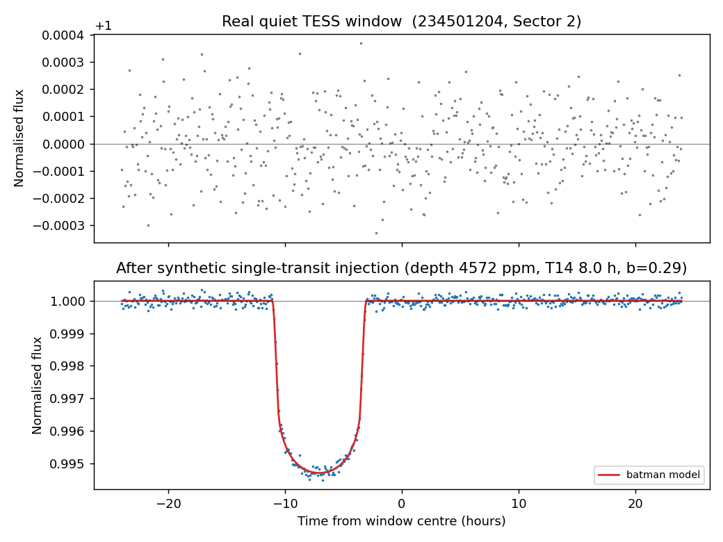
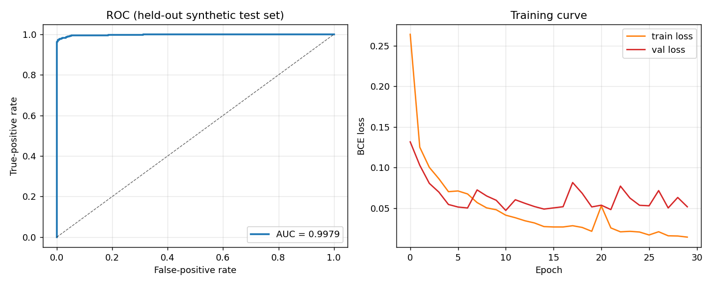
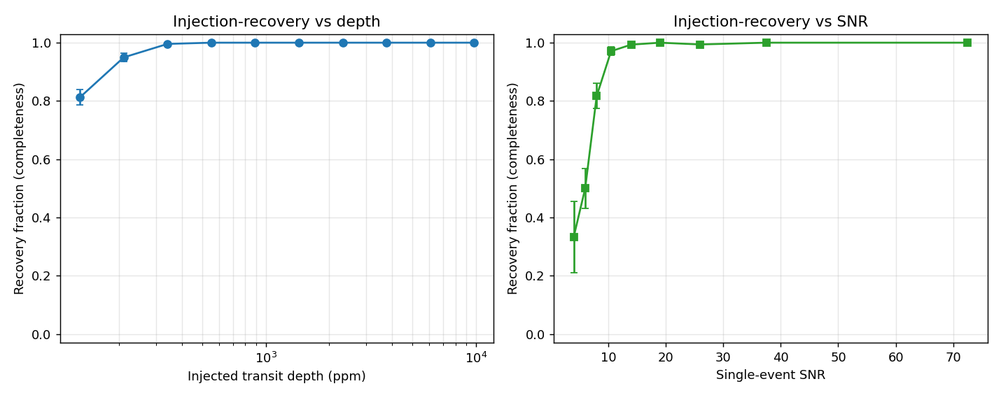
Standard transit search (Box-Least-Squares) assumes periodicity and requires at least two transits; a planet whose period exceeds the ~27-day TESS sector transits only once and is missed by automated pipelines — precisely the regime in which Planet Hunters TESS finds many of its discoveries. We train a 1-D convolutional neural network to recognise a single transit in a light-curve window, using synthetic injection: analytic transit signals from batman are injected into real, quiet TESS light curves to build an unlimited, perfectly labelled training set. On a held-out, star-disjoint synthetic test set the detector reaches ROC-AUC = 0.998. A full injection-recovery analysis quantifies completeness as a function of transit depth and signal-to-noise: recovery rises monotonically from ~33% at $\mathrm{SNR}=4$ to essentially 100% above $\mathrm{SNR}\approx15$ (depth $\gtrsim350$ ppm). The stellar backgrounds are real TESS data; the transits are synthetic, and any real-data detection is a candidate requiring standard vetting.

1. Introduction

The Box-Least-Squares algorithm ^[5] and its ML successors phase-fold a light curve on a trial period and require the transit to repeat. For a planet with orbital period longer than the observing baseline (a single 27-day TESS sector), only one transit occurs, so periodic search has nothing to fold and the event is discarded. These long-period systems are scientifically valuable — they probe cooler, wider orbits — and are exactly where citizen scientists (Planet Hunters TESS ^[6]) contribute most of their by-eye discoveries. On the automated side the problem is under-served. We treat single-transit detection as a supervised classification of light-curve windows, and solve the label-scarcity problem with synthetic injection.

2. Data

We use real TESS two-minute (SPOC) light curves obtained with lightkurve ^[4] for a set of 16 stars across multiple sectors (32 light curves in total). Each light curve is cleaned (NaN removal), normalised to fractional flux, flattened, and cut into two-day windows resampled to 512 points, yielding 324 real background windows. Crucially, the train/test split is by star (12 stars for training, 4 held out for testing) so that no star appears in both — a strict test of generalisation.

3. Methods

3.1 Synthetic transit injection

Positive examples are generated by injecting analytic single-transit signals into real quiet windows. The transit model is the Mandel & Agol (2002) formalism ^[3] as implemented in batman ^[2], with randomised depth (planet-to-star radius ratio, so depth $\delta\approx(R_p/R_\star)^2$), duration, impact parameter, and epoch within the window. Negatives are un-injected quiet windows and realistic artefacts. This yields an unlimited, perfectly labelled dataset: 6,000 training and 4,000 test examples, with injected transits spanning a broad signal-to-noise range (5th/50th/95th percentiles $\mathrm{SNR}=8.6/78/737$), where

$$\mathrm{SNR}\;\approx\;\frac{\delta}{\sigma}\,\sqrt{n_{\mathrm{in}}}$$

with $\sigma$ the per-point noise and $n_{\mathrm{in}}$ the number of in-transit points.

3.2 Classifier and evaluation

A 1-D CNN maps a 512-point window to the probability that it contains a single transit, trained with binary cross-entropy (Adam, 30 epochs, Apple-MPS). Performance is measured on the held-out, star-disjoint synthetic test set by ROC-AUC and by an injection-recovery analysis: the completeness (recovered fraction) as a function of injected transit depth and SNR, which is the standard way to characterise the sensitivity of a transit search.

4. Results

0.998

held-out ROC-AUC

97.7%

completeness @ FPR 0.016

6,000

injected train examples

16 / 32

stars / light curves

A real quiet TESS window before and after synthetic single-transit injection — **Figure 1.** The training signal. *Top:* a real quiet TESS window (TIC 234501204, Sector 2), scatter at the $\sim$100 ppm level. *Bottom:* the same window after injecting a synthetic single transit (depth 4572 ppm, duration 8 h, impact parameter 0.29); the batman analytic model (red) is overlaid on the injected data (blue). The backgrounds are real; the transits are synthetic and exactly labelled.

ROC curve on the held-out synthetic test set — **Figure 2.** Receiver-operating-characteristic curve on the held-out, star-disjoint test set (ROC-AUC = 0.998). At the chosen operating threshold the false-positive rate is 0.016 and the completeness is 0.977.

Injection-recovery: completeness versus transit depth and SNR — **Figure 3.** Injection-recovery. Completeness rises monotonically with signal strength — from ~33% at $\mathrm{SNR}=4$, through ~82% at $\mathrm{SNR}=8$, to essentially 100% above $\mathrm{SNR}\approx15$ — and with transit depth (81% at 131 ppm, 95% at 211 ppm, ~100% at $\gtrsim341$ ppm). This is the standard characterisation of a transit search's sensitivity, and its smooth, monotonic form is the expected, physically sensible behaviour.

5. Caveats

Transits are synthetic. The method is validated by injection-recovery; the stellar backgrounds are real TESS data, but the transits are simulated. Applying the trained detector to real data yields candidates, not detections.
A single event carries little information. Monotransits have no period and no second event to confirm them; the false-positive rate on real data is high (grazing eclipsing binaries, stellar variability, systematics). Strict vetting — odd/even and secondary-eclipse checks where possible, and neighbour-pixel analysis given TESS's ~21 arcsec pixels — is essential.
Small background sample. Sixteen stars is a modest diversity of real noise; a production search would draw backgrounds from thousands of stars across many sectors. The held-out scan here returned no candidates, as expected for so small a set.

6. Reproducibility

cd projects/p5-tess-monotransit
python3 src/monotransit_local.py   # downloads backgrounds, injects transits, trains, evaluates

Deterministic (seeded); runs locally on Apple M2 / MPS in about two minutes. Outputs: outputs/{injection_example,roc,recovery_curve}.png, candidates.csv, run_summary.json.

References

Ricker, G. R., et al. (2015). The Transiting Exoplanet Survey Satellite (TESS). JATIS 1, 014003. doi:10.1117/1.JATIS.1.1.014003.
Kreidberg, L. (2015). batman: BAsic Transit Model cAlculatioN in Python. PASP 127, 1161. doi:10.1086/683602 ; lkreidberg.github.io/batman.
Mandel, K., & Agol, E. (2002). Analytic Light Curves for Planetary Transit Searches. ApJ 580, L171. doi:10.1086/345520.
Lightkurve Collaboration (2018). Lightkurve: Kepler and TESS time series analysis in Python. ascl:1812.013. docs.lightkurve.org.
Kovács, G., Zucker, S., & Mazeh, T. (2002). A box-fitting algorithm in the search for periodic transits (BLS). A&A 391, 369. doi:10.1051/0004-6361:20020802.
Eisner, N. L., et al. (2021). Planet Hunters TESS I: results for the first two years. MNRAS 501, 4669. doi:10.1093/mnras/staa3739.