space-ml-lab · Project P4 · Technical report
Unsupervised Search for Anomalous Stellar Light Curves in TESS with a Convolutional Autoencoder
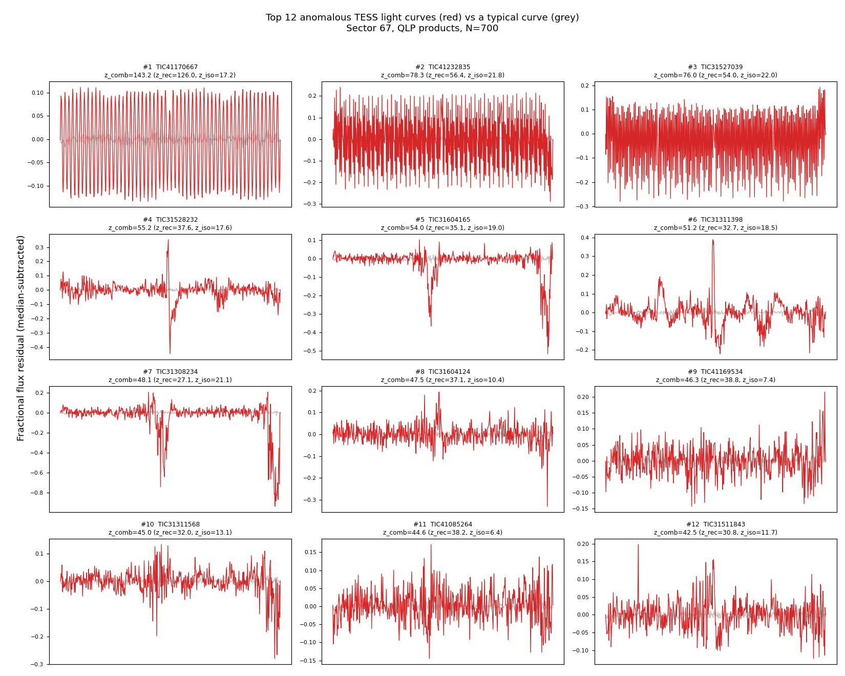
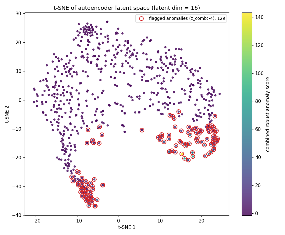
The overwhelming majority of machine-learning work on TESS light curves is supervised transit detection; genuine discoveries, however, often lie in the anomalous tail — objects that fit no template, such as the aperiodic deep dips of Boyajian's Star. We present a fully local, reproducible pipeline for unsupervised discovery of unusual light curves. A 1-D convolutional autoencoder learns a 16-dimensional representation of 700 real TESS QLP light curves; each object is then ranked by two complementary detectors — the autoencoder's reconstruction error (a deviation from the learned manifold of typical behaviour) and an Isolation Forest on the latent embeddings (structural isolation in the compressed space) — combined with robust median/MAD z-scores. The ranking cleanly surfaces high-amplitude periodic variables (eclipsing binaries and pulsators), deep isolated dips, and high-scatter stars; 129 of 700 objects exceed the anomaly threshold. All light curves are real; no results are fabricated.
1. Introduction
A supervised classifier can, by construction, only recover the classes it was trained on. For discovery — new variability, rare eclipses, instrumental pathologies, or genuinely novel behaviour — the objects of interest are precisely those absent from any label set. Unsupervised anomaly detection takes the opposite stance: it models the empirical distribution of "typical" light curves and quantifies deviation from it. The canonical motivation is KIC 8462852 (Boyajian's Star) [5], whose aperiodic, deep, irregular dimmings fit no known class and were found by human inspection. Automated, representation-based anomaly search over whole survey sectors is comparatively under-explored, and is well matched to the scale of TESS [1].
2. Data
We use QLP (Quick-Look Pipeline) high-level science products [3], compact FFI-derived light curves, retrieved through MAST with astroquery and read with lightkurve [2]. To obtain a well-defined, bounded sample of distinct stars we take a cone of radius $1.1^\circ$ centred on $(\alpha,\delta)=(90^\circ,-66.56^\circ)$ near the southern ecliptic pole, restricted to TESS Sector 67. Of 917 available products, 700 distinct light curves were downloaded (666 s, 8 parallel workers) and cached.
Each light curve is preprocessed to isolate shape from brightness and slow trends: remove NaNs; normalise to fractional flux ($\tilde f = f/\operatorname{median}f$); flatten by dividing out a wide running-median trend (window $\approx 10\%$ of the length) that removes instrumental drift while preserving sharp, deep astrophysical features; resample onto a uniform grid of $L=512$ points; and subtract the median so the baseline sits at zero.
3. Methods
3.1 Convolutional autoencoder
A 1-D convolutional autoencoder $f_\theta=g\circ h$ compresses each light curve $x\in\mathbb{R}^{L}$ to a latent code $z=h(x)\in\mathbb{R}^{d}$ with $d=16$ and reconstructs $\hat{x}=g(z)$. The encoder is three strided Conv1d blocks ($1\!\to\!16\!\to\!32\!\to\!64$, kernel 7, stride 2) followed by a linear bottleneck; the decoder mirrors it with transposed convolutions. It is trained purely self-supervised (no labels) to minimise the mean-squared reconstruction loss
$$\mathcal{L}(\theta)=\frac{1}{N}\sum_{i=1}^{N}\big\lVert x_i-\hat{x}_i\big\rVert_2^2,$$with Adam ($\text{lr}=10^{-3}$) for 120 epochs on the Apple-MPS backend. Because the bottleneck is narrow, the network can only learn the typical structure of the population; atypical light curves are reconstructed poorly, which is the anomaly signal.
3.2 Two-detector anomaly ranking
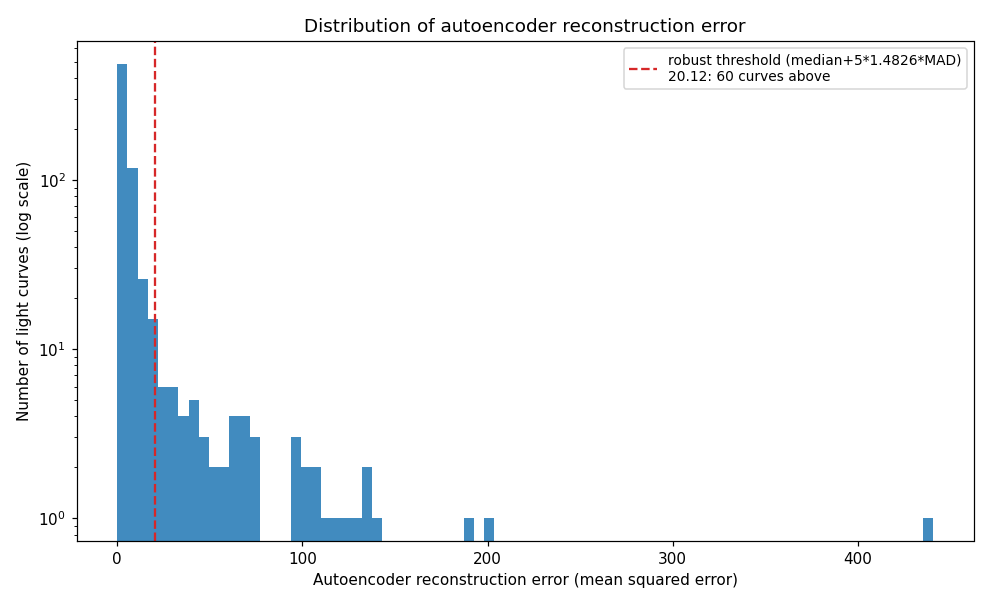
Reconstruction error: $e_i=\tfrac{1}{L}\lVert x_i-\hat{x}_i\rVert_2^2$ (deviation from the learned manifold in data space). Isolation Forest [4] (300 trees) is fit to the latent embeddings $\{z_i\}$; anomalies are isolated in fewer random splits, giving a score $s(z)=2^{-\,\mathbb{E}[h(z)]/c(n)}$ (isolation in latent space). The two independent signals are converted to robust median/MAD z-scores and summed,
$$Z(v)=\frac{v-\operatorname{median}(v)}{1.4826\,\operatorname{MAD}(v)},\qquad C_i=Z(e_i)+Z\!\big(s(z_i)\big),$$and objects are ranked by $C_i$. Using one detector in data space and one in latent space makes the ranking robust to the failure modes of either alone.
4. Results
Of the 700 objects, 129 exceed the combined-score threshold ($C_i>4$) and 60 exceed an independent robust reconstruction-error threshold. The top-ranked anomalies are visually and physically distinct from the flat, low-scatter typical curve.
The full ranking of all 700 objects is in outputs/anomaly_ranking.csv.
5. Caveats
- "Anomalous" means unusual, not new. The top objects are recognisable variable-star types and dippers — real, known classes that are simply rare or spectrally distinctive within this sample. The method ranks the unusual; it does not certify novelty.
- Artefacts dominate a real anomaly tail. Momentum-dump residuals, scattered light, edge effects, and blends populate the high-score list alongside astrophysical variability. This is a triage/ranking tool, not a discovery certificate.
- Vetting is required. Converting a ranked list into candidates needs cross-matching (SIMBAD, VSX, the TESS input catalogue), inspection of the target pixel files for blending, and ideally an active-learning loop to separate "interesting" from "instrumental".
6. Reproducibility
cd projects/p4-tess-weird-stars
python3 src/anomaly_search_local.py   # downloads QLP light curves, trains, ranks, writes figures
Deterministic (seeded); runs locally on Apple M2 / MPS. Outputs: outputs/{anomalies,recon_error_hist,latent_tsne}.png, anomaly_ranking.csv, run_summary.json.
References
- Ricker, G. R., et al. (2015). The Transiting Exoplanet Survey Satellite (TESS). JATIS 1, 014003. doi:10.1117/1.JATIS.1.1.014003.
- Lightkurve Collaboration (2018). Lightkurve: Kepler and TESS time series analysis in Python. Astrophysics Source Code Library, ascl:1812.013. docs.lightkurve.org.
- Huang, C. X., et al. (2020). Photometry of 10 Million Stars from the First Two Years of TESS Full-Frame Images (QLP). RNAAS 4, 204; and Kunimoto et al., extended-mission QLP releases. archive.stsci.edu/hlsp/qlp.
- Liu, F. T., Ting, K. M., & Zhou, Z.-H. (2008). Isolation Forest. IEEE ICDM, 413–422. doi:10.1109/ICDM.2008.17.
- Boyajian, T. S., et al. (2016). Where's the Flux? (KIC 8462852). MNRAS 457, 3988. doi:10.1093/mnras/stw218.
- Giles, D., & Walkowicz, L. (2019). Systematic serendipity: a test of unsupervised machine learning as a method for anomaly detection. MNRAS 484, 834. doi:10.1093/mnras/stz028.