space-ml-lab · Project P3 · Technical report

Deep-Learning Detection of Solar Radio Bursts in e-CALLISTO Dynamic Spectra

Enes  ·  Independent research project (space-ml-lab)

Draft — July 2026 · Code and data: space-ml-lab/projects/p3-solar-radio-bursts

1. Introduction

When magnetic reconnection accelerates electrons in the solar corona, the electrons excite plasma emission whose frequency tracks the local electron density. Because density falls with height, an outward-moving electron population emits at progressively lower frequencies, tracing a characteristic sloped feature in a dynamic spectrum (frequency versus time). The morphology encodes the physics: Type III bursts drift rapidly (their sources are near-relativistic electron beams), whereas Type II bursts drift slowly and mark a CME-driven shock, and Type IV bursts are broadband continua associated with the post-eruption phase ^[3]. Type II/IV activity therefore provides an early, ground-based signature of eruptions that may drive geomagnetic storms ^[6].

The e-CALLISTO network ^[1][2] is a global array of low-cost radio spectrometers that has monitored the Sun continuously since 2002, producing an open, multi-decade archive of dynamic spectra. Unlike gravitational-wave or fast-radio-burst data, on which thousands of machine-learning studies exist, ML applied to solar radio spectrograms is nascent (the first convolutional and object-detection studies appeared only in 2025–2026 ^[4]). This combination — a large, open, image-native archive in an under-explored modality, with freely available labels — is precisely the setting in which an individual can make a genuine contribution.

Contribution. We release a reproducible detection pipeline and an automatically labelled dataset derived from the e-CALLISTO burst lists, and we demonstrate that a compact CNN, trained on burst-centred crops, separates burst from quiet spectrograms with $\mathrm{AUC}\approx0.83$ on held-out data. We report the method transparently, including the preprocessing decision that was decisive for learning.

2. Data

2.1 Dynamic spectra

Each e-CALLISTO observation is a 15-minute FITS file storing a spectrogram of roughly $400\ \text{frequency channels}\times1800\ \text{time samples}$ (a time resolution of $\Delta t = 900\,\mathrm{s}/1800 = 0.5\,\mathrm{s}$), quantised to 8-bit flux density. Files are retrieved directly from the public archive:

http://soleil.i4ds.ch/solarradio/data/2002-20yy_Callisto/YYYY/MM/DD/
    STATION_YYYYMMDD_HHMMSS_NN.fit.gz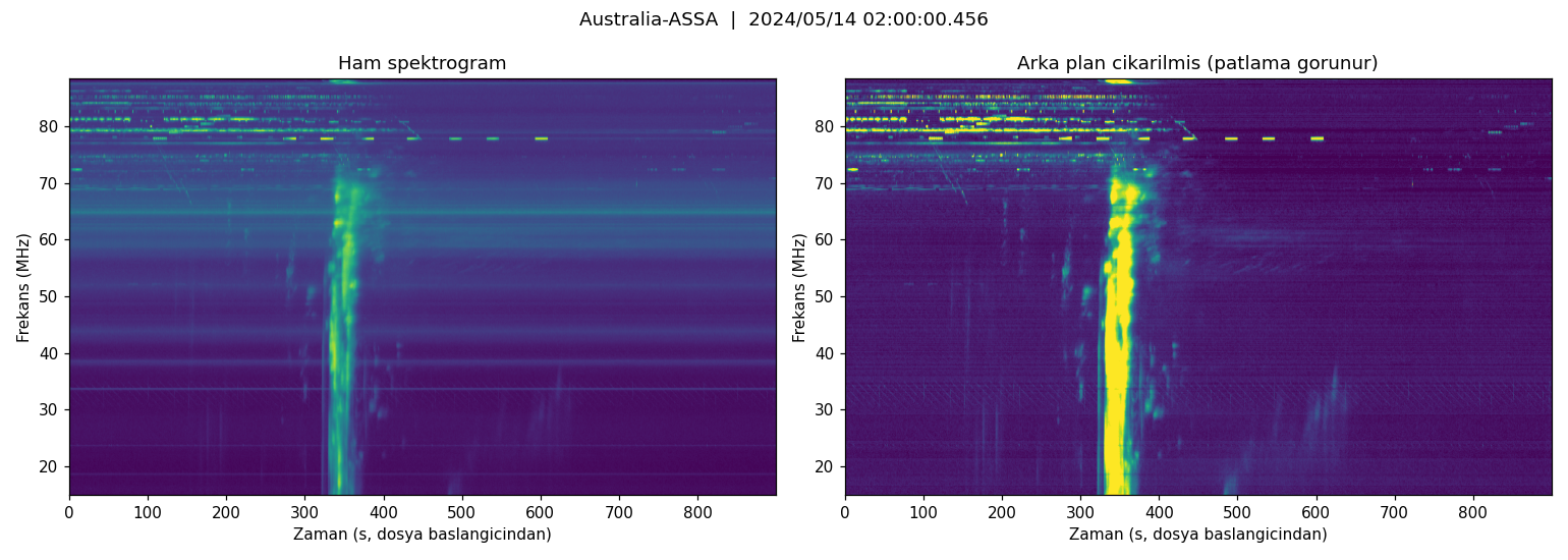

2.2 Labels from burst lists

The network publishes monthly, human-vetted burst lists giving the date, time span, burst type, and observing stations for every event:

#Date       Time          Type   Stations
20240501    10:47-10:55   III    BIR, GLASGOW, HUMAIN, SWISS-MUHEN, USA-BOSTON, ...
20240501    07:20-07:52   VI     AUSTRIA-UNIGRAZ, GERMANY-DLR, HUMAIN, INDIA-OOTY, ...

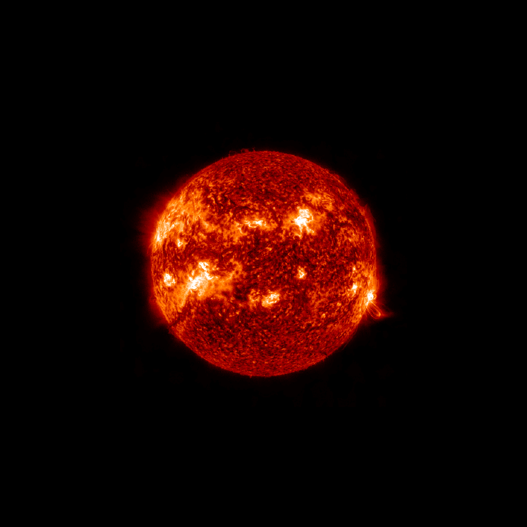
For May 2024 the list contains 387 records with type distribution III = 229, VI = 78, II = 22, IV = 8, and others. This period is deliberately chosen: the Sun was near solar-cycle-25 maximum, and the extreme storm of 10–14 May 2024 (the “Gannon storm”, including an X8.7 flare) produced abundant activity. We use three days (14–16 May 2024) and eight stations spanning a range of longitudes.

3. Methods

3.1 Automatic labelling

Each burst-list record specifies which stations observed the event and at what time. For a positive example we download the 15-minute file of a reporting station whose block contains the burst epoch. For negative (quiet-Sun) examples we sample 15-minute blocks that lie outside every listed burst window (with a $\pm300\,\mathrm{s}$ margin), from the same stations, so that positives and negatives share the same instruments and RFI environment and differ only in the presence of a burst.

3.2 Preprocessing and the cropping decision

The receiver's frequency response and slowly varying baseline are removed by subtracting, for each frequency channel $f$, the temporal median of that channel:

$$\tilde{S}(f,t) \;=\; S(f,t) \;-\; \operatorname{median}_{t'} S(f,t') \tag{1}$$

followed by 2nd–98th-percentile clipping and min–max scaling to $[0,1]$.

A Type III burst lasts only seconds, whereas a file spans 900 s. Feeding the whole file and resizing to $128\times128$ shrinks the burst to $\sim\!1$–2 pixels, and a classifier trained this way never rises above chance ($\mathrm{AUC}\approx0.52$). We therefore crop a window of $W = 180\,\mathrm{s}$ centred on the catalogued burst epoch (a random window of the same width for negatives), so the burst fills the frame:

$$c = \left\lfloor (t_0 - t_{\text{block}})/\Delta t \right\rceil,\qquad \text{crop} = \tilde{S}\!\left[\,:,\; c-\tfrac{W}{2\Delta t}\; :\; c+\tfrac{W}{2\Delta t}\,\right] \tag{2}$$

where $t_0$ is the burst start and $t_{\text{block}}$ the file's start time. Each crop is resized to $128\times128$. This single change is what makes the problem learnable (§4).

3.3 Model and training

The classifier is a compact CNN: four $3\times3$ convolutional blocks ($16\!\to\!32\!\to\!64\!\to\!64$ channels), each with batch normalisation ^[5], ReLU, and max-pooling, followed by global average pooling, dropout ($p=0.3$), and a single logit. It is trained with the Adam optimiser ^[5] ($\text{lr}=10^{-3}$) for 15 epochs. To counter the class imbalance ($N_+ < N_-$) we use a weighted binary cross-entropy,

$$\mathcal{L} \;=\; -\frac{1}{N}\sum_{i=1}^{N}\Big[\, w_{+}\,y_i \log \sigma(z_i) \;+\;(1-y_i)\log\big(1-\sigma(z_i)\big)\Big],\qquad w_{+}=\frac{N_-}{N_+} \tag{3}$$

with $z_i$ the network logit and $\sigma$ the logistic function. Training runs on the laptop's GPU via PyTorch's Metal (MPS) backend.

4. Results

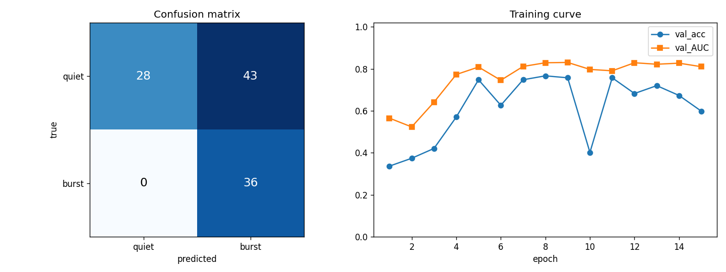
The dataset comprises 535 crops (135 burst, 400 quiet) from eight stations over three days. With the burst-centred crop, the held-out (20%) ranking performance reaches $\mathrm{AUC}\approx0.83$, compared with $\approx0.52$ for the whole-file baseline — a direct demonstration that the informative signal is the localised burst, not the global spectrogram.

5. Discussion and limitations

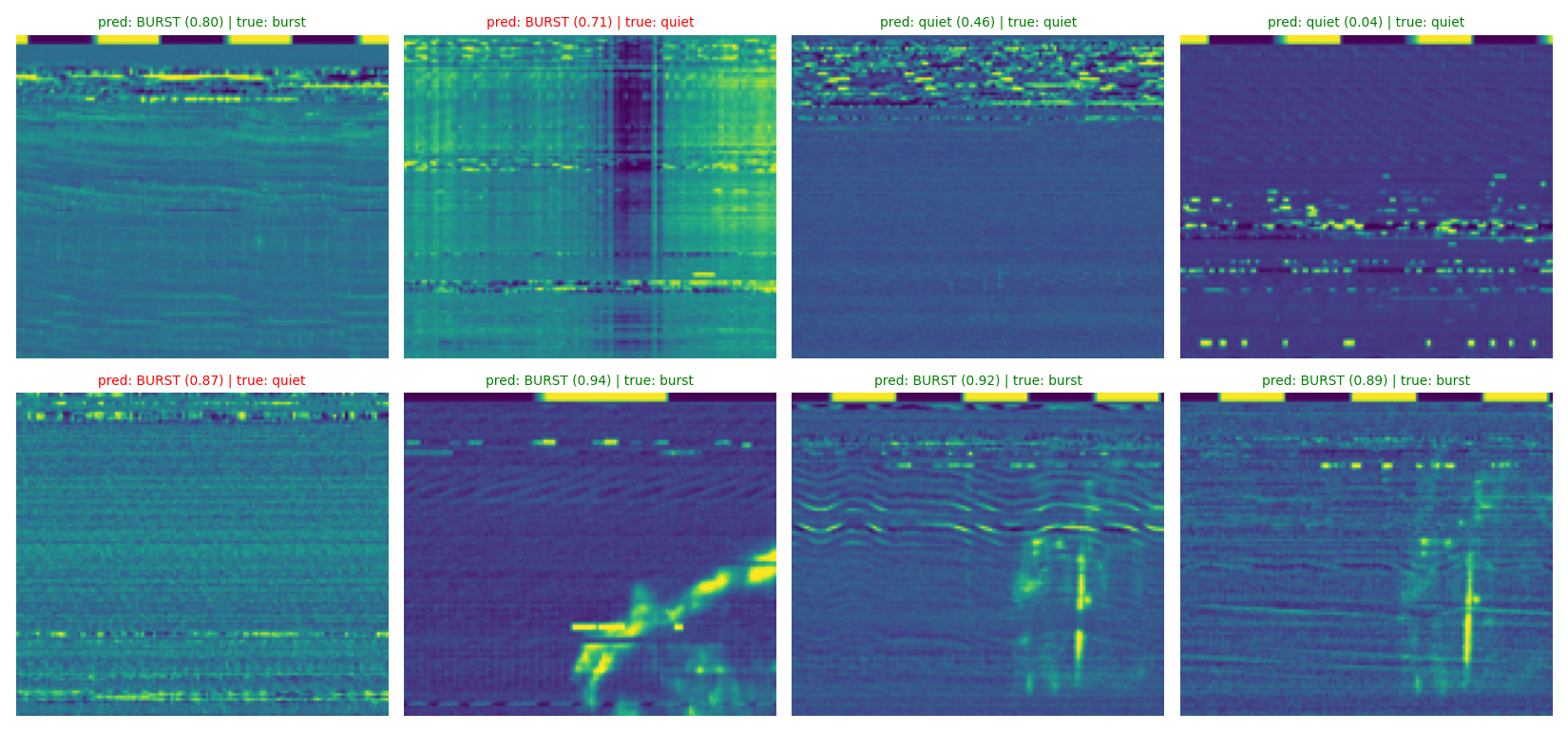
False positives from RFI. The main errors are broadband or bright interference features misread as bursts. Enriching the negative set with diverse RFI, and adding Grad-CAM attribution to confirm the model attends to the burst rather than horizontal RFI lines, are immediate next steps.

Label imprecision. Burst-list times are given to the minute, so the true burst may sit up to $\pm60\,\mathrm{s}$ from the crop centre; the $180\,\mathrm{s}$ window is chosen to tolerate this.

Class imbalance. Type III dominates; rarer, science-critical Type II/IV events are few, which will require targeted sampling or synthetic augmentation for the type-classification stage.

Scope. This is a burst/quiet detector, not yet a discovery instrument. It is an honest first result, not a confirmed scientific claim.

6. Next steps

1. Type classification (III/II/IV/V/VI) using the labels already present in the burst list, with class weighting.
2. Grad-CAM interpretability to verify physically meaningful attention.
3. Cross-modal space-weather prediction — regressing the contemporaneous NOAA GOES X-ray flare class, or the subsequent Kp/Dst geomagnetic index, from the radio spectrogram. This is the genuinely novel, under-explored contribution.
4. Release the labelled dataset and trained model with a Zenodo DOI and a Research Note of the AAS.

7. Reproducibility

All results here were produced by src/train_local.py on an Apple M2. The data are public; the labels are the e-CALLISTO burst lists. To reproduce:

cd projects/p3-solar-radio-bursts
python3 src/train_local.py        # downloads data, builds the labelled set, trains, saves figures

Outputs: data/dataset.npz, models/burst_cnn.pt, outputs/results.png, outputs/example_predictions.png. A Colab notebook (notebooks/solar_radio_burst_detector.ipynb) reproduces the same pipeline in the cloud.

---

References

- A. O. Benz, C. Monstein, H. Meyer et al. (2009). A World-Wide Net of Solar Radio Spectrometers: e-CALLISTO. Earth, Moon, and Planets 104, 277–285. doi:10.1007/s11038-008-9267-6.
- The e-CALLISTO network — International Network of Solar Radio Spectrometers. http://www.e-callisto.org/ (data archive: soleil.i4ds.ch/solarradio).
- Classification of solar radio bursts (Types I–V), after J. P. Wild and the Zurich/ETH scheme; see e.g. M. J. Reid & H. S. Ratcliffe (2014), A review of solar type III radio bursts, Res. Astron. Astrophys. 14, 773. arXiv:1404.6117.
- Recent machine-learning studies of e-CALLISTO spectra (2025–2026), including CNN and object-detection (YOLO) burst detection and transfer-learning for Type II/III identification; e.g. arXiv:2512.11487.
- S. Ioffe & C. Szegedy (2015), Batch Normalization, arXiv:1502.03167; D. P. Kingma & J. Ba (2015), Adam: A Method for Stochastic Optimization, arXiv:1412.6980.
- NOAA Space Weather Prediction Center — GOES X-ray flux and geomagnetic indices. https://www.swpc.noaa.gov/.