space-ml-lab · Project P2 · Technical report
Unsupervised Anomaly Detection in Low-Resolution Spectra: A Self-Supervised Autoencoder with Isolation-Forest Latent Scoring
The most scientifically valuable objects in a spectroscopic survey are, by definition, those that fit no template. We present a compact, fully local pipeline for unsupervised discovery: a self-supervised autoencoder learns a 16-dimensional representation of real spectra, and anomalies are ranked by combining the reconstruction error with an Isolation Forest on the latent embeddings. The method is designed for SPHEREx (NASA, launched March 2025), whose all-sky near-infrared spectra are a natural target but whose extracted-spectrum catalogues are not yet public; we therefore develop and validate the identical pipeline on 4,990 genuine SDSS DR17 optical spectra as a documented stand-in. Without using labels, the latent space spontaneously organises by object class, and the anomaly ranking is strongly enriched in extreme-emission-line objects: 96% of the top-100 anomalies carry emission-line/broad-line subclasses versus 30.9% of the parent sample — a $3.1\times$ enrichment. All data are real.
1. Introduction
Supervised classification can only recover the classes it was trained on. For discovery — rare transients, blends, mis-calibrated sources, or genuinely new spectral types — the interesting objects are precisely those absent from any label set, so a classifier cannot surface them. Unsupervised anomaly detection takes the opposite stance: it models the empirical distribution of "typical" spectra and quantifies deviation from it, an approach that has repeatedly proven productive on spectroscopic surveys [4][3][7]. This is especially timely for SPHEREx, which measures a low-resolution spectrum ($0.75$–$5\,\mu$m, 102 channels) at every point on the sky and whose source catalogues are not yet released — untouched ground for a representation-learning / anomaly layer [1].
2. Data
The final sample is drawn from SDSS DR17 [5] SpecObj requiring zWarning=0, snMedian>5, sciencePrimary=1; a modular-hash ordering scatters the selection across plates and sub-surveys. Each spectrum is resampled by linear interpolation onto a common grid of 512 points uniform in $\log_{10}\lambda$ over 3850–9000 Å. The cached sample (data/spectra.npz) contains 4,990 spectra spanning $z\in[-0.002, 6.9]$:
| class | count | fraction |
|---|---|---|
| GALAXY | 2,830 | 56.7% |
| STAR | 1,500 | 30.1% |
| QSO | 660 | 13.2% |
3. Methods
Let a spectrum be a flux vector $x\in\mathbb{R}^{D}$ with $D=512$.
3.1 Preprocessing
To separate spectral shape from brightness, each spectrum is divided by its mean flux, $\tilde{x}=x/\bar{x}$; each wavelength bin is then standardised across the sample,
$$x^{\mathrm{std}}_{ij}=\frac{\tilde{x}_{ij}-\mu_j}{\sigma_j},\qquad \mu_j=\tfrac{1}{N}\sum_i \tilde{x}_{ij},\quad \sigma_j^2=\tfrac{1}{N}\sum_i(\tilde{x}_{ij}-\mu_j)^2.$$3.2 Self-supervised autoencoder
An autoencoder $f_\theta=g\circ h$ compresses each standardised spectrum to a latent code $z=h(x)\in\mathbb{R}^{d}$ with $d=16$ and reconstructs $\hat{x}=g(z)$, trained purely self-supervised (no labels) to minimise the mean-squared reconstruction loss
$$\mathcal{L}(\theta)=\frac{1}{N}\sum_{i=1}^{N}\big\lVert x_i-\hat{x}_i\big\rVert_2^2.$$The encoder is $512\to256\to128\to16$ and the decoder its mirror, with ReLU activations; Adam ($\text{lr}=10^{-3}$, weight decay $10^{-5}$), 200 epochs, batch size 256, on the Apple-MPS backend (seconds of wall-clock). Final train / validation MSE: 0.127 / 0.196 (standardised units).
3.3 Anomaly scores
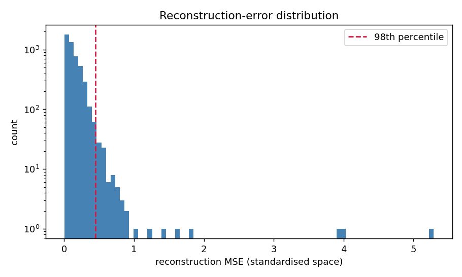
Reconstruction error. $e_i=\tfrac{1}{D}\lVert x_i-\hat{x}_i\rVert_2^2$ — large $e_i$ means the model, trained on the typical population, cannot represent this spectrum (an outlier in data space).
Isolation Forest in latent space [2]. 300 random trees are fit to $\{z_i\}$; anomalies are isolated in fewer splits, i.e. shorter expected path length. The score is
$$s(z)=2^{-\,\mathbb{E}[h(z)]\,/\,c(n)},\qquad c(n)=2H(n-1)-\frac{2(n-1)}{n},$$with $H$ the harmonic number; $s\to1$ indicates a strong anomaly.
Combined ranking. The two independent signals are converted to robust median/MAD $z$-scores and summed, $C_i=Z(e_i)+Z(s(z_i))$ with $Z(v)=(v-\mathrm{median}(v))/(1.4826\,\mathrm{MAD}(v))$. Using one detector in data space and one in latent space makes the ranking robust to the failure modes of either alone.
4. Results
Emergent class structure (unsupervised). Although no labels were used in training, a t-SNE [6] projection of the 16-D latent space cleanly separates stars, galaxies, and quasars into distinct regions — direct evidence that the autoencoder learned a physically meaningful representation. The flagged anomalies concentrate in the sparse, peripheral regions (the outskirts of the quasar locus and the galaxy–quasar transition), exactly where an anomaly detector should place them.
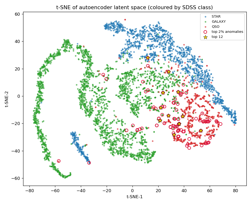
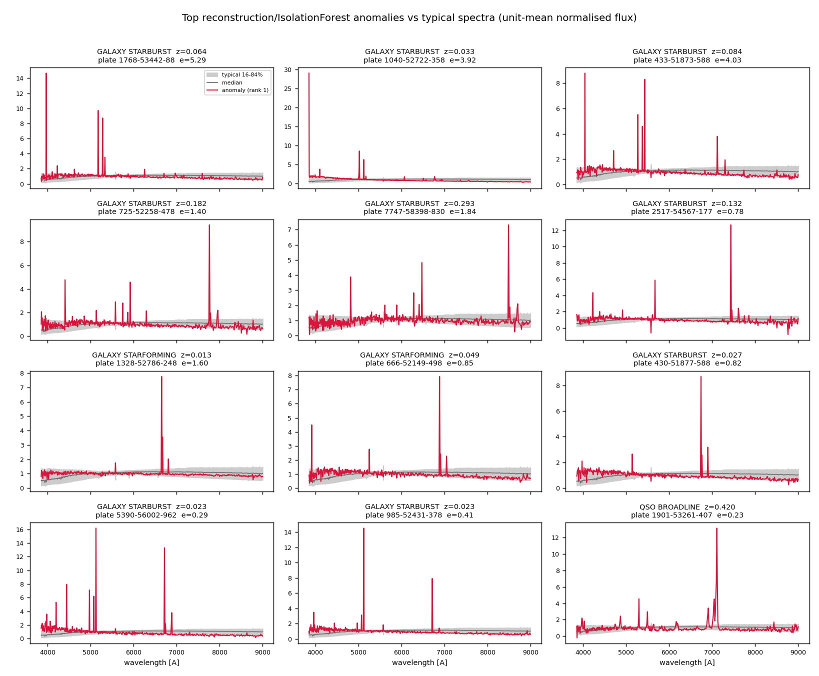
What the anomalies are. Of the 100 top-ranked anomalies, 68 are galaxies and 32 are quasars, with no ordinary stars; 96 of 100 carry an emission-line or broad-line subclass (STARBURST, STARFORMING, BROADLINE, AGN), versus 30.9% of the full sample — a $3.1\times$ enrichment. This is physically sensible: the bulk population is dominated by smooth absorption/continuum spectra, so the objects most unlike the bulk are those with towering [O III], H$\alpha$, [O II] or broad quasar lines.
4.1 Top-ranked anomalies
| rank | class | subclass | $z$ | recon. err |
|---|---|---|---|---|
| 1 | GALAXY | STARBURST | 0.064 | 5.29 |
| 2 | GALAXY | STARBURST | 0.033 | 3.92 |
| 3 | GALAXY | STARBURST | 0.084 | 4.03 |
| 7 | GALAXY | STARFORMING | 0.013 | 1.60 |
| 12 | QSO | BROADLINE | 0.420 | 0.23 |
Full ranking of all 4,990 sources in outputs/anomaly_ranking.csv.
5. Caveats
- "Anomaly" means rare, not new. The top anomalies are recognisably extreme-emission-line galaxies and quasars — real, known types that are under-represented and spectrally distinctive. The method ranks the unusual; it does not certify novelty.
- Most anomalies in a real survey are artefacts (flux-calibration residuals, blends, sky-subtraction, edges). This is a triage / ranking tool; human vetting and active learning [4] are required to convert a ranked list into discoveries.
- Stand-in data. The specific anomalies are SDSS optical objects, not SPHEREx NIR sources. The results validate the method; applying it to SPHEREx requires the forced-spectrophotometry extraction step (§2).
- Normalisation dependence. The outlier set depends on the chosen normalisation; unit-mean + per-bin standardisation emphasises spectral shape.
6. Reproducibility
cd projects/p2-spherex-anomaly
python3 src/fetch_sdss.py            # query + download + resample -> data/spectra.npz
python3 src/anomaly_detect_local.py  # autoencoder + isolation forest -> figures + ranking
Deterministic (seeded); runs locally on Apple M2 / MPS.
References
- Doré, O., et al. (SPHEREx Collaboration). SPHEREx: An All-Sky Near-Infrared Spectral Survey. NASA/JPL. spherex.caltech.edu — IRSA: irsa.ipac.caltech.edu/Missions/spherex.html.
- Liu, F. T., Ting, K. M., & Zhou, Z.-H. (2008). Isolation Forest. IEEE ICDM, 413–422. doi:10.1109/ICDM.2008.17.
- Portillo, S. K. N., Parejko, J. K., Vergara, J. R., & Connolly, A. J. (2020). Dimensionality Reduction of SDSS Spectra with Variational Autoencoders. AJ 160, 45. doi:10.3847/1538-3881/ab9644.
- Baron, D., & Poznanski, D. (2017). The weirdest SDSS galaxies: results from an outlier detection algorithm. MNRAS 465, 4530–4555. doi:10.1093/mnras/stw3021.
- Abdurro'uf, et al. (2022). The Seventeenth Data Release of the Sloan Digital Sky Surveys (DR17). ApJS 259, 35. doi:10.3847/1538-4365/ac4414.
- van der Maaten, L., & Hinton, G. (2008). Visualizing Data using t-SNE. JMLR 9, 2579–2605.
- A search for anomalies in the DESI spectra with variational autoencoders (2025). arXiv:2506.17376.