Jet tagging · GNN case study · Technical report
When Does a Graph Neural Network Beat a Permutation-Invariant Baseline? A Jet-Tagging Case Study
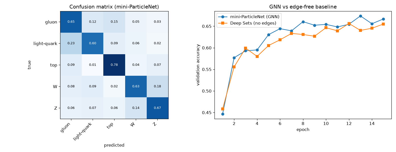
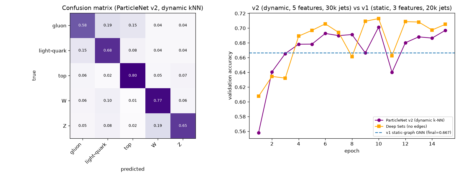
We compare a dynamic-graph, k-nearest-neighbour Graph Neural Network (a reproduction of the defining trait of ParticleNet [1]) against a Deep Sets [2] baseline with no edges at all, on five-class jet tagging (gluon, light-quark, top, W, Z) using the JetNet dataset [3]. Two versions are reported. In v1 (a static, fully-connected graph, 3 raw features, 20,000 jets) the GNN edges provide a small but real gain (66.7% vs. 65.5% accuracy). In v2 (a genuinely dynamic k-NN graph rebuilt at every layer in learned feature space, 5 engineered features, 30,000 jets) the GNN does not beat its own, stronger Deep Sets baseline (69.7% vs. 70.5%). We report both results honestly: the v1$\to$v2 accuracy gain came almost entirely from feature engineering, not from the graph edges, and we discuss the likely reasons -- small point clouds (30 particles), a modest training budget, and a genuinely strong baseline. The physics is consistent throughout: confusion is concentrated exactly where domain knowledge predicts (gluon/light-quark, W/Z), evidence that both models learn real structure even where the GNN's architectural advantage does not materialise.
1. Introduction
A jet -- the collimated spray of particles produced when a quark or gluon hadronises -- is naturally represented as an unordered particle cloud: a variable-size set of particles with no canonical ordering. Graph Neural Networks that build a k-nearest-neighbour graph over this cloud and pass messages along its edges (ParticleNet [1] being the landmark method) are the standard architecture for jet tagging. A natural question, and the one this report answers empirically, is how much of a GNN's performance actually comes from the edges themselves, as opposed to a good per-particle representation pooled without any relational structure at all (Deep Sets [2]).
2. Data
JetNet [3] provides particle clouds (up to 30 constituents per jet) for five jet types: gluon, light-quark, top, W, and Z, with per-particle $(\eta^{\text{rel}}, \phi^{\text{rel}}, p_T^{\text{rel}})$ and a validity mask. v1 uses 20,000 jets (4,000/class) and the 3 raw features; v2 uses 30,000 jets (6,000/class) and 5 engineered features (see §3.3).
3. Methods
3.1 Deep Sets baseline (no edges)
A per-particle MLP $\phi$ is applied independently to every particle, then pooled by mean and max across the jet, and classified by a small head $\rho$:
$$y = \rho\big(\,\mathrm{mean}_i\,\phi(x_i)\ \Vert\ \mathrm{max}_i\,\phi(x_i)\,\big).$$This is permutation-invariant by construction and uses no information about how particles relate to one another -- only their individual features.
3.2 EdgeConv and dynamic graphs
The core GNN layer, EdgeConv [1], updates each particle's representation using its k nearest neighbours:
$$\mathbf{x}_i' = \max_{j\in\mathcal{N}(i)}\ \mathrm{MLP}\big(\,[\,\mathbf{x}_i\ ,\ \mathbf{x}_j-\mathbf{x}_i\,]\,\big).$$The neighbour set $\mathcal{N}(i)$ carries the relational information Deep Sets lacks: the $\mathbf{x}_j - \mathbf{x}_i$ term is a relative feature (a local geometric/learned-space relationship), not just a per-particle one. In v1 this graph is static: fully-connected and fixed for the whole forward pass. In v2, following real ParticleNet, the k-NN graph is dynamically rebuilt at every layer in that layer's own learned feature space (k=16), so deep layers can connect particles that are spatially distant but representationally similar -- the defining "Dynamic Graph CNN" property.
3.3 Engineered features (v2 only)
v2 augments the 3 raw features with two standard derived quantities: $\log(p_T^{\text{rel}})$ and $\Delta R = \sqrt{(\eta^{\text{rel}})^2+(\phi^{\text{rel}})^2}$, giving 5 features per particle for both the GNN and its Deep Sets baseline (a fair comparison).
4. Results
4.1 v1 -- static graph, 3 features, 20k jets
Here the static-graph GNN provides a small, real edge over Deep Sets.
4.2 v2 -- dynamic k-NN graph, 5 features, 30k jets
Moving from v1 to v2, overall accuracy improved by roughly 5 points -- but the dynamic-graph GNN did not beat its own (stronger) Deep Sets baseline. The gain is attributable almost entirely to the engineered features, not to the graph edges.
4.3 The physics is consistent throughout
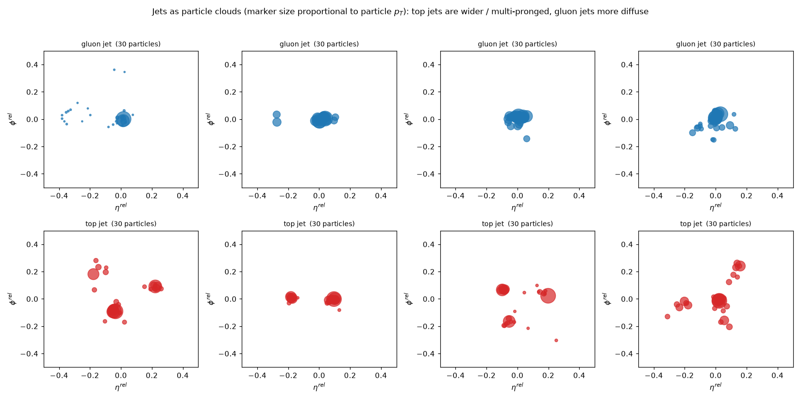
In both versions, confusion concentrates exactly where domain knowledge predicts: gluon and light-quark jets are frequently confused with each other (a famously hard discrimination in the jet-tagging literature), and W and Z are confused with each other (near-degenerate mass, both two-pronged). Top jets are the easiest class (highest recall in both versions) because their three-body decay gives a distinctive multi-pronged topology (Figure 1). This consistency is evidence that both models are learning genuine physical structure, even in the configuration where the GNN's architectural advantage does not show up in the headline accuracy.
5. Discussion: why didn't the dynamic graph win?
- Small point clouds. With only 30 particles per jet, $k=16$ nearest neighbours is already close to a fully-connected graph -- there is limited "dynamic" structure left to exploit. ParticleNet's advantage is better documented on jets with 100-150 constituents.
- Modest training budget. 15 epochs and an untuned learning rate is a small budget for a higher-capacity model; the GNN's validation curve is visibly less converged than the Deep Sets curve (Figure 3).
- A genuinely strong baseline. Deep Sets with well-engineered features is a competitive, well-documented baseline in the jet-tagging literature, not a strawman.
6. Reproducibility
python3 src/jet_tagging_local.py            # v1: static fully-connected graph
python3 src/jet_tagging_particlenet_v2.py   # v2: dynamic k-NN graph + engineered features
Data: JetNet [3] (pip install jetnet). Runs on CPU (Apple M2); GPU is not required at this scale. Outputs: outputs/{example_jets,results,results_v2}.png, outputs/run_summary{,_v2}.json.
7. A next step, if resumed
Retry on JetNet150 (150 particles/jet), where dynamic k-NN graphs have real geometric structure to exploit, with more epochs and a learning-rate schedule -- or use weaver-core [4], the training framework behind the published ParticleNet numbers (approximately 90%+ accuracy).
References
- Qu, H., & Gouskos, L. (2020). ParticleNet: Jet Tagging via Particle Clouds. Phys. Rev. D 101, 056019. arXiv:1902.08570 · github.com/hqucms/ParticleNet.
- Zaheer, M., et al. (2017). Deep Sets. NeurIPS 2017. arXiv:1703.06114.
- Kansal, R., et al. JetNet. github.com/jet-net/JetNet · Zenodo (JetNet150).
- Qu, H. weaver-core — the HEP training framework behind published ParticleNet results. github.com/hqucms/weaver-core.
- Fey, M., & Lenssen, J. E. (2019). Fast Graph Representation Learning with PyTorch Geometric. arXiv:1903.02428 · pytorch-geometric.readthedocs.io.